---

Monte Carlo for Risk Management: VaR and ES

---

Modeling Stock Prices with Geometric Brownian Motion

In the realm of finance, the Geometric Brownian Motion (GBM) model serves as a fundamental tool for simulating and analyzing the behavior of stock prices over time. This model is based on the concept that stock prices evolve stochastically, influenced by drift and volatility.
The GBM model is represented by the following stochastic differential equation: \[ dS_t = \mu S_t dt + \sigma S_t dW_t \]
where:
- \(S_t\) is the stock price at time \(t\)
- \(\mu\) is the drift (expected return)
- \(\sigma\) is the volatility (standard deviation of returns)
- \(dW_t\) is a Wiener process (Brownian motion) increment
The discretized version for discrete time steps can be written as: \[ S_{t+1} = S_t \exp\left((\mu - \frac{1}{2} \sigma^2) \Delta t + \sigma \sqrt{\Delta t} Z_t\right) \]
where:
- \(\Delta t\) is the time step
- \(Z_t\) is a random variable sampled from a standard normal distribution

Value at Risk (VaR)

Value at Risk (VaR) is a risk assessment measure that quantifies the potential loss an investment might face over a specified time horizon at a given confidence level. In the context of the GBM model, VaR is calculated based on the simulated final prices. The \(1 - \alpha\) quantile of these prices represents the maximum potential loss with a confidence level of \(\alpha\). \[ \operatorname{VaR}_\alpha(X)=-\inf \left\{x \in \mathbb{R}: F_X(x)>\alpha\right\}=F_Y^{-1}(1-\alpha) \]

Conditional Value at Risk (CVaR)

Conditional Value at Risk (CVaR), also known as expected shortfall, provides an additional layer of risk assessment beyond VaR. It represents the average value of the losses that exceed the VaR at a specified confidence level. Mathematically, CVaR is calculated as the average of all prices that fall below the VaR. \[ \mathrm{ES}_\alpha(X)=-\frac{1}{\alpha} \int_0^\alpha \operatorname{VaR}_\gamma(X) d \gamma \]

Python Implementation

To put the theory into practice, let's implement the GBM model using Python. We'll use historical stock price data for Apple and simulate potential price paths. Then, we'll calculate VaR and CVaR based on the simulated outcomes.

import pandas as pd
import numpy as np
import matplotlib.pyplot as plt
import yfinance as yf

data = pd.DataFrame(yf.download('AAPL', 
                                start='2021-01-01', 
                                end='2022-01-01')['Close'])
data ['return'] = np.log(data / data.shift())

plt.figure()
data.plot(subplots=True)

S0 = data['Close'].iloc[-1]
r = data['return'].mean()
sigma = data['return'].std()
I =1000
T = 252
S = np.zeros((T+1, I))
S[0] = S0
for t in range(1,T+1):
    S[t] = (S[t-1] * np.exp(r - .5 * sigma **2 + 
            sigma * np.random.standard_normal(I)))
            
plt.figure()
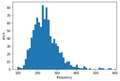
plt.hist(S[-1], bins=50)             
plt.xlabel('frequency')
plt.ylabel('price')

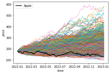
data = pd.DataFrame(yf.download('AAPL',start='2022-01-01')['Close'])[:253]

plt.figure()
plt.plot(data.index,S, alpha=.5)
plt.plot(data, '-k', lw=2, label='Apple')
plt.xlabel('time')
plt.ylabel('price')
plt.legend()

    
# VaR and CVaR
S_f = S[-1]
S_f.sort()
alpha = 0.05  
VaR = -np.percentile(S_f, 100 * alpha) + S0
CVaR = -np.mean([s - S0 for s in S_f if s-S0 <= -VaR])

print('Value at Risk (VaR) at %.0f %% confidence level: %.2f' 
      %(100-alpha*100, VaR)) 
print("Conditional Value at Risk (CVaR) at %.0f %% confidence level: %.2f"
      %(100-alpha*100, CVaR))

Value at Risk (VaR) at 95 % confidence level: 22.06
Conditional Value at Risk (CVaR) at 95 % confidence level: 36.22
So, with 95% confidence the loss per share will be above $22.06 and if it is more it is expected to be on average $36.22.