---

Markowitz's Efficient Frontier and Portfolio Diversification

---

Modern portfolio theory

Markowitz’s modern portfolio theory formulates portfolio optimization problem considering only mean and variance excluding higher moments. This optimization problem can be written as the following utility maximization with risk aversion coefficient \(\lambda\):

Equivalently one can find minimum variance for a given expected return:

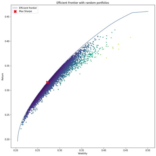
The solution of the first optimization problem for all risk aversions or the second one for all returns gives us an efficient frontier of portfolios.

Python Implementation

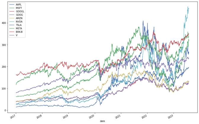
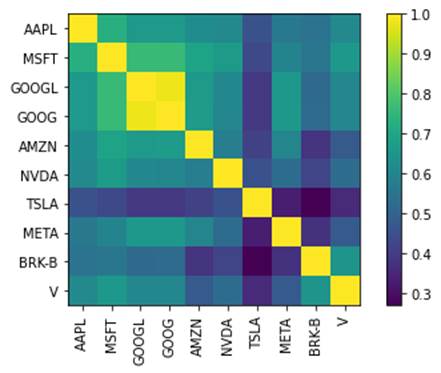
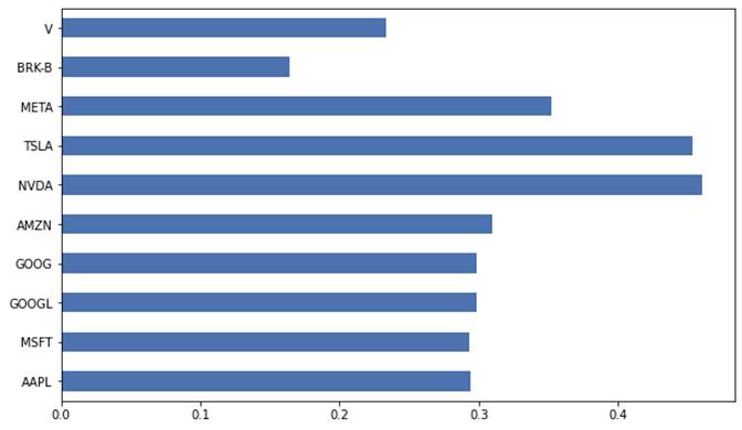
Here we consider a portfolio of 10 stocks with the highest market cap in S&P 500. First, we download and store prices, and make some plotes. From the price history plots and correlation heatmap we can see that the returns are quite highly correlated. also we see the expected returns of the individual stocks are not much different. the portfolio of the stocks are not very good for diversification. We can see that the stocks are big tech stocks. We should choose stocks from different industries so hopefully we get lower correlations.

import pandas as pd
import numpy as np
import matplotlib.pyplot as plt
from pypfopt import risk_models
from pypfopt import plotting
from pypfopt import expected_returns
from pypfopt.efficient_frontier import EfficientFrontier
from pypfopt.discrete_allocation import DiscreteAllocation, get_latest_prices

portfolio = pd.read_csv("prices.csv",parse_dates=True,index_col="date")

plt.figure()
# portfolio[portfolio.index >= "2021-04-01"].plot(figsize=(15,10));
portfolio.plot(figsize=(15,10))

sample_cov = risk_models.sample_cov(portfolio, frequency=252)

S = risk_models.CovarianceShrinkage(portfolio).ledoit_wolf()

plt.figure()
plotting.plot_covariance(S, plot_correlation=True);

mu = expected_returns.capm_return(portfolio)

plt.figure()
mu.plot.barh(figsize=(10,6));

Regardless, let's see how we can solve for optimal portfolio:

ef = EfficientFrontier(mu, S)
weights = ef.max_sharpe()

cleaned_weights = ef.clean_weights()
print(dict(cleaned_weights))

ef.portfolio_performance(verbose=True)



latest_prices = get_latest_prices(portfolio)

da = DiscreteAllocation(weights, latest_prices, total_portfolio_value=100000)

# Number of shares of each stock to purchase
allocation, leftover = da.greedy_portfolio()
print("Discrete allocation:", allocation)
print("Funds remaining: {:.2f}".format(leftover))

n_samples = 10000
w = np.random.dirichlet(np.ones(len(mu)), n_samples)
rets = w.dot(mu)
stds = np.sqrt((w.T * (S @ w.T)).sum(axis=0))
sharpes = rets / stds

print("Sample portfolio returns:", rets)
print("Sample portfolio volatilities:", stds)

# Plot efficient frontier with Monte Carlo sim
ef = EfficientFrontier(mu, S)

fig, ax = plt.subplots(figsize= (10,10))
plotting.plot_efficient_frontier(ef, ax=ax, show_assets=False)

# Find and plot the tangency portfolio
ef2 = EfficientFrontier(mu, S)
ef2.max_sharpe()
ret_tangent, std_tangent, _ = ef2.portfolio_performance()

# Plot random portfolios
ax.scatter(stds, rets, marker=".", c=sharpes, cmap="viridis_r")
ax.scatter(std_tangent, ret_tangent, c='red', marker='X',s=150, label= 'Max Sharpe')

# Format
ax.set_title("Efficient Frontier with random portfolios")
ax.legend()
plt.tight_layout()
plt.show()

The results give us the optimized portfolio weights and the expected return and volatility of the portfolio:

{'AAPL': 0.10022, 'MSFT': 0.10013, 'GOOGL': 0.10001, 'GOOG': 0.10033, 'AMZN': 0.09986, 'NVDA': 0.10063, 'TSLA': 0.10029, 'META': 0.10031, 'BRK-B': 0.09827, 'V': 0.09994}

Expected annual return: 31.6%

Annual volatility: 27.2%

Sharpe Ratio: 1.09

Further Reading

• Kelliher, C., 2022. Quantitative Finance with Python: A Practical Guide to Investment Management, Trading, and Financial Engineering. CRC Press.
• https://www.analyticsvidhya.com/blog/2023/06/optimizing-portfolios-with-the-mean-variance-method-in-python/#:~:text=The%20mean%2Dvariance%20method%20is,return%20while%20minimizing%20its%20variance.