---

Extreme Value Theory: Probability of Future Losses

---

Extreme Value Theory (EVT)

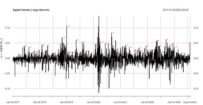
Estimating the probabilities of extreme losses are important in risk management. Extreme Value Theory says that the extreme tail of many distributions can be described by the Generalized Pareto Distribution (GPD). First we need to standardize our returns:

\[z_{t+1}=R_{P F, t+1} / \sigma_{P F, t+1} \stackrel{\text { i.i.d. }}{\sim} D(0,1)\] The distribution of observations beyond the threshold y converges to Generalized Pareto Distribution: \[G P D(y ; \xi, \beta)= \begin{cases}1-(1+\xi y / \beta)^{-1 / \xi} & \text { if } \xi>0 \\ 1-\exp (-y / \beta) & \text { if } \xi=0\end{cases}\]

Estimating the Tail Index Parameter, \(\xi\)

In risk management \(\xi\) is positive and we can use the Hill estimator:

\[F(y)=1-c y^{-1 / \xi} \approx 1-(1+\xi y / \beta)^{-1 / \xi}=G P D(y ; \xi, \beta)\]

The likelihood function for all \(y_i\) greater than \(u\):

\[L=\prod_{i=1}^{T_u} f\left(y_i\right) /(1-F(u))=\prod_{i=1}^{T_u} \frac{1}{\xi} c y_i^{-1 / \xi-1} /\left(c u^{-1 / \xi}\right), \quad \text{for} \quad y_i>u\]

The log-likelihood:

\[\ln L=\sum_{i=1}^{T_u}\left(-\ln (\xi)-(1 / \xi+1) \ln \left(y_i\right)+\frac{1}{\xi} \ln (u)\right)\]

Therefore, maximizing the log-likelihood, i.e., setting the derivative with respect to \(\xi\) gives us the Hill estimator for the tail index parameter:

\[\xi=\frac{1}{T_u} \sum_{i=1}^{T_u} \ln \left(y_i / u\right)\]

For \(c\) we can write:

\[F(u)=1-c u^{-1 / \xi}=1-T_u / T\]

Solving for \(c\):

\[c = \frac{T_u}{T} u^{1/\xi}\]

R Implementation

In the following code we use Apple returns from 2017 onward. Using the Block Maxima Method we find maximum monthly losses. Using maximum-likelihood estimator for the parameters of the generalized extreme value distribution in the end gives us the distribution fitted to our data.

# libraries
library(xts) 
library(qrmdata)
library(qrmtools)
library(zoo)
library(rugarch)
library(tidyquant)

aapl <- tq_get('aapl',
               from = "2017-01-01",
               get = "stock.prices")

aapl = read.zoo(aapl[,c('date','close')])

# plot
plot(aapl, main='apple price history', xlab='Date', ylab='close price')

# returns
returns=returns(aapl)
L <- -returns

# plot losses (negative returns)
plot(L, main = "S&P 500 losses (-log-returns)",
         xlab = "Time t", ylab = expression(L[t] == -log(S[t]/S[t-1])))

# Block Maxima Mehod
# monthly maxima
monthly.maxima <- period.apply(L, INDEX = endpoints(L, "months"), FUN = max) 

# add scatter plot
lines(monthly.maxima,type='p',col='red')

# fit GEV distribution
fit <- fit_GEV_MLE(monthly.maxima)
(xi <- fit$par[["shape"]])
(mu  <- fit$par[["loc"]])
(sig <- fit$par[["scale"]])
fit$SE 

the probability that next month's maximal risk-factor change  exceeds all previous ones and the 1-year return level or the loss expected to be exceeded once every 12 months:

# probability of max risk factor exceeding next month
1-pGEV(max(head(monthly.maxima,  n = -1)), 
       shape = xi,  loc = mu,  scale = sig)

# return level in a year or the loss expected to exceed 
qGEV(1-1/12, shape = xi, loc = mu, scale = sig)

References

• Christoffersen, P., 2011. Elements of financial risk management. Academic press.
• McNeil, A.J., Frey, R. and Embrechts, P., 2015. Quantitative risk management: Concepts. Economics Books.
• https://en.wikipedia.org/wiki/Extreme_value_theorem
• https://georgebv.github.io/pyextremes/user-guide/3-block-maxima/