---

Introduction to Decision Trees with Python Implementation

---

Decision Tree Learning

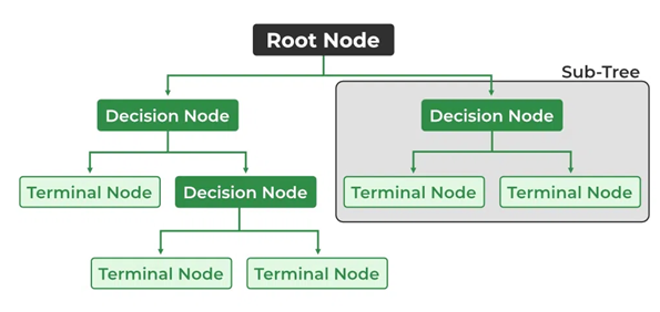
Decision tree learning is a supervised machine learning method used in statistics and data mining. It involves creating a predictive model in the form of a classification or regression tree based on a set of observations. Classification trees are used when the target variable has discrete values, representing class labels, while regression trees are employed for continuous values. Decision trees are popular for their simplicity and intelligibility. They visually represent decisions and decision-making processes, making them useful in decision analysis. In data mining, decision trees describe data, and the resulting classification tree can be used for decision-making.

Decision tree learning is widely used in data mining is aiming to create a predictive model for a target variable based on multiple input variables. In this context, a decision tree is a straightforward representation used for classifying examples. Assuming finite discrete domains for input features and a single target feature called "classification," the decision tree comprises nodes labeled with input features and branches labeled with possible values of the target feature.

The tree-building process involves recursively splitting the source set into subsets based on classification features, creating internal nodes and decision paths. This top-down induction of decision trees is a greedy algorithm, where each node is split to maximize predictive value. The recursion stops when subsets have uniform values for the target variable, or further splitting adds minimal predictive value.

The data consists of records in the form \((\mathbf{x}, Y) = (x_1, x_2, x_3, ..., x_k, \, Y)\) , where \(Y\) is the target variable, and \(\mathbf{x}\) is the feature vector used for the task.

Types of Decision Trees

Decision trees used in data mining can be categorized into two main types:

• Classification Tree: This type predicts the class (discrete) to which the data belongs. Each leaf node in the tree represents a class label, and the branches represent conjunctions of features leading to those labels.
• Regression Tree: This type predicts outcomes that can be considered real numbers, such as the price of a house or a patient's length of stay in a hospital.

The term Classification and Regression Tree (CART) refers to both procedures, and it was introduced by Breiman et al. in 1984. While classification and regression trees share similarities, there are differences, particularly in the procedure used to determine where to split.
Ensemble methods, known as boosted trees and bagged decision trees, construct multiple decision trees for improved performance:

• Boosted Trees: Incrementally builds an ensemble by training each new instance to emphasize the training instances previously mis-modeled. AdaBoost is a typical example, applicable to both regression and classification problems.
• Bootstrap Aggregated (Bagged) Decision Trees: Builds multiple decision trees by repeatedly resampling training data with replacement, and the trees vote for a consensus prediction.
• Random Forest Classifier: A specific type of bootstrap-aggregated decision trees.
• Rotation Forest: Each decision tree is trained by first applying principal component analysis (PCA) on a random subset of the input features.

Notable decision tree algorithms include ID3 (Iterative Dichotomiser 3), C4.5 (a successor of ID3), and CART (Classification And Regression Tree). These algorithms were developed independently but follow a similar approach for learning decision trees from training tuples.

Additionally, concepts from fuzzy set theory have been proposed for a special version of a decision tree known as Fuzzy Decision Tree (FDT), where an input vector is associated with multiple classes, each having a different confidence value. Boosted ensembles of FDTs have been suggested for improved performance.

Let’s take a brief look at two algorithms in the following.

Let’s take a brief look at two algorithms in the following.

ID3 Algorithm

The ID3 algorithm begins with the original set \(S\) as the root node. On each iteration of the algorithm, it iterates through every unused attribute of the set (\S\) and calculates the entropy \(H(S)\) or the information gain \(IG(S)\) of that attribute. It then selects the attribute which has the smallest entropy (or largest information gain) value. The set \(S\) is then split or partitioned by the selected attribute to produce subsets of the data.

in summary:

a) Take the Entire dataset as an input.
b) Calculate the Entropy of the target variable, As well as the predictor attributes
c) Calculate the information gain of all attributes.
d) Choose the attribute with the highest information gain as the Root Node
e) Repeat the same procedure on every branch until the decision node of each branch is finalized.

Entropy is a measure of impurity or disorder in a set of examples. In the context of decision trees, it is used to quantify the uncertainty associated with a given set of data. \[\mathrm{H}(S)=\sum_{x \in X}-p(x) \log _2 p(x)\] Information gain measures the effectiveness of an attribute in reducing uncertainty (entropy) about the classification of the data. \[I G(S, A)=\mathrm{H}(S)-\sum_{t \in T} p(t) \mathrm{H}(t)=\mathrm{H}(S)-\mathrm{H}(S \mid A)\]

Classification And Regression Tree Algorithm

The CART (Classification And Regression Tree) algorithm is a decision tree algorithm that can be used for both classification and regression tasks. It was introduced by Leo Breiman and his colleagues in 1984. CART is widely used due to its simplicity, effectiveness, and versatility in handling different types of data. Here's an overview of how the CART algorithm works:
Basic Steps of the CART Algorithm:

• Binary Splitting: The CART algorithm builds a binary tree, where each node represents a binary decision based on the value of a particular attribute. At each node, the algorithm selects the attribute and a corresponding threshold that best splits the data into two subsets.
• Objective Function for Splitting: For classification tasks, the Gini impurity is commonly used as an objective function to measure the impurity of a node. For regression tasks, the mean squared error (MSE) is used to evaluate the variance of the target variable within a node.
• Node Splitting: The algorithm evaluates all possible splits for each attribute and selects the split that minimizes the Gini impurity (for classification) or the mean squared error (for regression). The selected attribute and threshold are used to create two child nodes, and the data is divided accordingly.
• Recursion: The process is repeated recursively for each child node until a stopping criterion is met. This could be a predefined tree depth, a minimum number of samples in a node, or other criteria.
• Leaf Node Prediction: When a stopping criterion is met, a leaf node is created. For classification, the majority class in the node is assigned to the leaf. For regression, the mean or median of the target values in the node is used.

Gini Impurity

Gini impurity is used by the CART (classification and regression tree) algorithm for classification trees. Gini impurity measures how often a randomly chosen element of a set would be incorrectly labeled if it were labeled randomly and independently according to the distribution of labels in the set. It reaches its minimum (zero) when all cases in the node fall into a single target category.
\[\mathrm{I}_G(p)=\sum_{i=1}^J\left(p_i \sum_{k \neq i} p_k\right)=\sum_{i=1}^J p_i\left(1-p_i\right)=\sum_{i=1}^J\left(p_i-p_i^2\right)=\sum_{i=1}^J p_i-\sum_{i=1}^J p_i^2=1-\sum_{i=1}^J p_i^2\]

Python Implementation

We will use the following model from sklearn library to predict the price direction for bitcoin.

sklearn.tree.DecisionTreeClassifier

class sklearn.tree.DecisionTreeClassifier(*, criterion='gini', splitter='best', max_depth=None, min_samples_split=2, min_samples_leaf=1, min_weight_fraction_leaf=0.0, max_features=None, random_state=None, max_leaf_nodes=None, min_impurity_decrease=0.0, class_weight=None, ccp_alpha=0.0)

The following Python code implements a basic trading strategy using Backtrader, a financial analysis library. The strategy employs a Decision Tree classifier to make buy and sell decisions based on historical price data for Bitcoin (BTC-USD). The strategy's features include the price difference between close and open, Relative Strength Index (RSI), and trading volume over a specified lookback period. The Decision Tree model is trained on these features, and predictions are made to determine whether to buy, sell, or hold. The strategy uses a simple position sizing approach and executes trades accordingly. The Backtrader engine is configured to handle the strategy, and the code concludes by printing the initial and final values of the brokerage account and plotting the strategy's performance over the specified historical data period.

import backtrader as bt
from sklearn.tree import DecisionTreeClassifier
import numpy as np
import pandas as pd
import yfinance as yf
import matplotlib.pyplot as plt

class MLStrategy(bt.Strategy):
    params = (
        ("lookback_period", 30),
        ("decision_tree_model", DecisionTreeClassifier())
    )

    def __init__(self):
        self.data_close = self.datas[0].close
        self.data_open = self.datas[0].open
        self.decision_tree_model = self.params.decision_tree_model
        self.lookback_period = self.params.lookback_period
        self.rsi = bt.indicators.RelativeStrengthIndex(self.data_close, period=14)
        self.volume = self.datas[0].volume
        self.order = None

    def next(self):
        if len(self) > self.lookback_period:
            # Convert array.array to NumPy arrays for subtraction
            close_prices = np.array(self.data_close.get(size=self.lookback_period))
            open_prices = np.array(self.data_open.get(size=self.lookback_period))
            price_diff = close_prices - open_prices
            rsi_values = np.array(self.rsi.get(size=self.lookback_period))
            volume_values = np.array(self.volume.get(size=self.lookback_period))
            
            # Feature generation
            features = np.column_stack((price_diff, rsi_values, volume_values))

            # Decision tree input
            X = features.reshape(-1, 3)

            # price directions
            y = np.sign(np.diff(self.data_close.get(size=self.lookback_period + 1)))
          
            # Train the decision tree model
            self.decision_tree_model.fit(X[:-1], y[1:])

            # Predict using decision tree
            prediction = self.decision_tree_model.predict(X[-1:])

            # Check if there is no open position
            if not self.position:
                cash = self.broker.get_cash()
                asset_price = self.data.close[0]
                position_size = cash / asset_price * 0.99

                # Make trading decision based on prediction
                if prediction[-1] == 1:
                    self.buy(size=position_size)
            else:
                if prediction[-1] == -1:
                    self.close()

    def notify_order(self, order):
        if order.status in [order.Submitted, order.Accepted]:
            return

        # Check if an order has been completed
        if order.status == order.Completed:
            if order.isbuy():
                self.log(f"Buy executed: {order.executed.price:.2f}")
            elif order.issell():
                self.log(f"Sell executed: {order.executed.price:.2f}")

        # Reset order
        self.order = None

    def log(self, txt, dt=None):
        dt = dt or self.datas[0].datetime.date(0)
        print(f"{dt.isoformat()}, {txt}")

if __name__ == '__main__':
    # Create a Cerebro engine
    cerebro = bt.Cerebro()

    # Add data
    data = bt.feeds.PandasData(dataname=yf.download('BTC-USD', 
                                                    period='3mo',
                                                    ))

    cerebro.adddata(data)

    # Add the strategy
    cerebro.addstrategy(MLStrategy)

    # Set the initial cash amount
    cerebro.broker.setcash(100.)
    cerebro.broker.setcommission(.001)

    print(' Brokerage account: $%.2f' % cerebro.broker.getvalue())
    cerebro.run()
    print(' Brokerage account: $%.2f' % cerebro.broker.getvalue())

    # Plot the strategy
    plt.rcParams["figure.figsize"] = (10, 6)
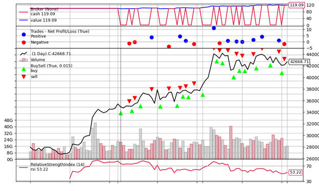
    cerebro.plot()